J. W. Wright, M. T. Rietveld, F. T. Berkey, N. A. Zabotin
Ionograms as presented on the Web by the dynasonde real-time analysis system («AutoDSND») require from you some accommodation and familiarity, which it is the purpose of these notes to provide.
The present description applies specifically to real-time Web presentations by dynasondes operating at Tromsø Norway (EISCAT), Kiruna, Sweden (IRF) and previously on Svalbard by EISCAT and at Utah State University's Bear Lake Observatory, and Lycksele Sweden (IRF).
It is useful to bear in mind that dynasonde ionogram images are merely graphical representations of numerical data. They provide an aide-memoir of ionospheric conditions, and on occasion a basis for questioning or confirming some subsequent analysis steps (e.g. N(h) inversion, or critical-frequency values), but the ionogram images should not be mistaken as the source of data for subsequent study.
Most ionogram modes of the dynasonde obtain data over a wide range of radio frequency in «pulsets», each of which is a small group of pulses (currently 8 at Tromsø, 4 at Bear Lake), carefully planned to sample closely spaced times, antennas and radio-frequency offsets or «delta-f». Receiver complex-amplitude output is sampled frequently (e.g., at 10μs intervals) in each such «channel», throughout a wide range of echo delay, whether or not echoes are present. The samples are processed by one or another method of echo recognition and noise rejection, yielding a fairly compact raw recording of single complex amplitude values (those nearest the amplitude-modulus peak) for each echo, of each pulse, antenna, and delta-f channel. The dynasonde has two receivers, so, for example, 8 pulses provide 16 channels of complex-amplitude data, or 32 real data.
For the modes just described (those having file names with extensions «.B_G») the method of echo recognition (Wright and Pitteway, 1979) occurs in real time (a time of the order of the pulset, .08s) within the dynasonde computer, by a process ("PEAKS") of range coincidence: echo amplitude peaks are detected within the complex-amplitude samples by a 5 or 7-point algorithm. Putative echoes from each of the n pulses of the pulset are compared for coincidence within a small tolerance, and those which yield n «hits» are accepted as genuine echoes. In some modes, m hits (with n > m) are accepted. For m = n, and n = 4 the probability of accepting a false echo is less than 10-4. (The pulset with n = 8 is about equally effective, since impulsive noise is highly correlated between the two receivers). The process does, however, discard some genuine echoes; in particular, this happens when two echoes are somewhat overlapped, and when their relative phases are not nearly opposite, whereupon their amplitude modulus may resemble a broad plateau, or a peak plus a plateau.
Another echo recognition method («PRETEC») is under development (Wright, and Pitteway, 1999), and runs occasionally as an experiment at Tromsø (file name extension «.BPG»). Before describing it, a discussion of the information content of pulsets is useful.
At Tromsø, an 8-pulse set («pulset») and a 6-antenna receiving array are used. (Bear Lake uses a 4-pulse set and 4 receiving antennas. These differences mainly affect parameter accuracy, but not basic capabilities. We continue this discussion using the Tromsø example). With two parallel receivers in the dynasonde, there are a total of 16 complex-amplitude channels (32 real, dependent variables) plus the independent variables of time t, frequency f, antenna location (X, Y or East, North) and antenna orientation (Eastward, Northward), for each recognized echo. In addition, there are receiver attenuation values (multiples of 4 dB steps dynamically assigned per pulset), which are needed to recover the full 160 dB dynamic range of the system. The channels are sampled at 10μs intervals (1.5 km of range delay) during a chosen interval, usually 70 - 800 km after the transmitted pulse (for ionospheric work). In addition, a few samples taken before pulse transmission are used to characterize the prevailing radio noise at the particular frequency of the pulse.
This information comprises the totality of a dynasonde ionogram, albeit in very raw and obscure form. (A simple plot of echo-selected sampling time vs radio frequency resembles a classical analog ionogram, unless you look too closely). The information is transformed by an algorithm appropriate to the pulset design (Pitteway and Wright, 1982), into six phase-dependent quantities, plus an error quantity, plus an echo-peak amplitude (plus the aforementioned noise sample):
These eight primary quantities, in ensemble, are «the echo», in dynasonde ideology. Various secondary quantities (e.g., echo zenith and azimuth directions) are also obtained.
The eight items of the list above are mainly dependent on phase differences among the independent variables of time, antenna and frequency (but they include also the mean phase, and peak amplitude). We may put them to work in a different way: they comprise a set of properties that serve to distinguish genuine echoes from impulsive noise.
When the transformation algorithm, which yields the first eight echo attributes above, is applied successively to each of the 10-μs complex amplitude samples, nonsense values are obtained for each quantity except where an echo is present. (Of course, a reasonable value may occur by chance for a single attribute, but the chance of this occurring for all attributes in concert is very low. More important, within an echo, the successive attribute values are comparatively stable. These properties can be exploited to recognize the echo itself, and to distinguish it from impulsive nose. This is the basis for PRETEC (Wright and Pitteway, 1999). We have found that echo discrimination does not depend critically on the stability tolerances, and that stability over at least four 10-μs complex amplitude samples is sufficient to increase the echo count by about 60% compared to the echo «peaks» method. The additional echoes are mainly those which, because of range proximity to other echoes, do not yield distinct amplitude peaks. Furthermore, the echo attributes can now be represented with greater accuracy by their weighted-means over the stable samples, using the local echo amplitudes as weights.
Evidently, PRETEC requires all of the information of a pulset, but no more than that. If the dynasonde operating system («FAIS») could deliver individual pulsets to the data analysis computer (e.g., at 0.08s intervals), PRETEC could accomplish its task easily within that time, so that the full ionogram would be represented by its selected echoes and all of their physical attributes, fully classified, within .08s of the ionogram end. However, revisions of FAIS are not undertaken lightly, and at present PRETEC runs only after completion of the full, un-examined, data acquisition process; such recordings, some 30 MB in length, would set a minimum of about two minutes between «real time» ionograms. At Tromsø at most one such recording (file extension «.BPG») is obtained each hour, and after PRETEC the 30MB raw recording is not archived.
Dynasonde recordings using the older, standard «PEAKS» method of echo recognition (file extension «.B_G») are typically less than 100 kB in length.
Many subsequent analyses are performed using selections of the primary physical data (irrespective of the echo recognition and parameterization method), among which we mention:
Before plotting R′(f), the ionogram echoes have self-associated into dynamic classes or «traces'. The present classification procedure works as follows: Imagine the echoes in a sequential list, ordered according to radio frequency or time of acquisition (either will do). At any point in the list, the attributes of a «new» echo j are compared with average values of the attributes for each already-recognized trace. The averages are maintained in such a way that they describe the current end of the trace. The best match of the new echo to the existing traces is identified, and if the match is "good enough", the echo joins that trace, meanwhile updating the trace-attribute mean vales. If the new echo fails to match within selected tolerances, a new trace is started. This association process has the useful feature that echo attributes can «evolve» smoothly within each trace.
This section title is quite conventional for analysis of ionosonde data, but from the viewpoint of dynasonde methods it is becoming obsolete. The term «N(h) profile inversion» recalls the one-dimensional formulation by which traditional methods assumed vertical propagation of sounding signals. The most popular of these methods is well-known as «POLAN» [Titheridge, 1985].
The assumption of vertical propagation was quite natural to methods ininitially designed for manually scaled analog ionograms, which recorded only the dependence of group-path time vs. radio frequency. The Dynasonde, however, is equipped with a small spaced-antenna system; with sophisticated analysis of pulse phase information, it provides directions of arrival for each radio echo, together with accurate group propagation time (virtual range, R') and other quantities described elsewhere in this tutorial. Such results show that vertical propagation is in fact a relatively rare event. 3D illustrations of echolocations accompany every ionogram on this Website, revealing actual properties of the local three-dimensional plasma density distribution. A new inversion procedure is required to recover this information.
One principle limitation of a three-dimensional inversion algorithm is the local character of ionosonde measurements: they provide the perspective from a single ground location, in contrast to radio tomography. The 3D ionogram inversion problem may be formulated as the recovery of pre-defined model parameters that describe both vertical and horizontal gradients of ionospheric plasma density. A «Wedge-Stratified Ionosphere» (WSI) model is the appropriate substitution for the former «Plane-Stratified Ionosphere» model. In the WSI, plasma density surfaces are represented locally at a sequence of ranges by tilted sections of «frame» planes; the density between two frame planes (inside a «wedge») depends only on the angle between them.
A full-scale inversion algorithm (NeXtYZ, or «next wise») recovers the complete set of WSI parameters, equivalent to the altitude dependence of local horizontal gradients. A somewhat simplified version («NeXtYZ Lite») approximates with constant (but different) tilts for the E and F regions, incidentally permitting a more realistic treatment of magnetic-field direction in the problem.
Determination of the WSI model parameters proceeds upward in slant range and consecutively from the bottom of the ionosphere, in a sequence of thin layers. By a principal novelty of the NeXtYZ approach, each wedge is determined using multiple numerical ray tracings in combination with least-squares group range residual minimization. The power of modern PCs is utilized to a full extent. Aside from the solution of the main inversion task, this approach yields the real spatial positions of reflection for all legitimate ionogram echoes.
It is well known that without correction for the following situations, ionogram inversions cannot be considered correct:
Among other innovations of NeXtYZ are treatments of the underlying ionization and valley problems based on the latest physical models [Titheridge 2000, 2004]. The models used by NeXtYZ are not constant and arbitrary; they contain adjustable parameters which are influenced by effects of valley and underlying ionization on the echoes observed from the overlying regions. The principal such effect is the differential retardation imposed on Ordinary and eXtraordinary echoes. If both polarizations are observed at radio frequencies fairly close to the corresponding unobserved plasma frequencies, they are used by NeXtYZ to constrain the model parameters. These remarks pertain to the advantage of NeXtYZ when given just the right information obtainable from a good, but simple, ionogram.
Identifying and selecting the «right information» from a complicated ionogram (and ionograms are often complicated) is a separate and prior problem. Examples may be found where automated trace selection fails to represent prevailing conditions. NeXtYZ offers built-in protections for more robust operation of the automated analysis. In particular, the full NeXtYZ analysis is less sensitive to trace selection because it treats all meaningful traces according to their respective echolocations. The usual action of the method in these situations is to increase the error estimates of the resulting profile.
The ionogram images presented on the Web have now dropped the POLAN profile inversion, and instead present the results of a Full-3D NeXtYZ calculation. (POLAN and the 'Lite' version of NeXtYZ were both presented for comparison on these images from 19 February through 20 October 2005).
In contrast to POLAN, where the results were traditionally described as "vertical profiles" whether or not echolocation information was compatible with this assumption, the NeXtYZ profiles really are a best estimate of the vertical profile, obtained as the plasma frequency variation along a vertical line through the ensemble of wedge stratifications.
Note that the NeXtYZ profiles (thin continuous red line in the log-log R(fp) frame) are now accompanied by vertical error bars. These error estimates combine the basic errors of group-range estimation (proportional to EP, plotted at the bottom of the lower panel of the images), with the least-squares residual arising from the representation by a single wedge containing the reflection points of its defining group of echoes. In most cases, the residual contributes much more than the EP-dependent error.
For an individual echo occurring by total internal reflection, the plasma frequency at reflection is given absolutely for Ordinary polarization by the radio frequency itself, and can be considered free of error for any practical purpose. For echoes of eXtraordinary polarization, the plasma frequency is related to the radio frequency by fp = sqrt(fx(fx - fH)), where fH is the electron gyrofrequency at the reflection height. NeXtYZ uses for fH an extrapolated ground value (according to a dipole field law), and this is a potential source of error in attributing a value of fp to the error-free value of fx.
The vertical error bars given on the NeXtYZ profiles reflect the facts that in ionograms, radio frequency (and, for practical purposes, the reflection plasma frequency) is the absolutely-known independent variable, while the group range R', and the inverted true range R, are subject to measurement and representation errors. Depending on the local slope (dR/dfp) of the profile at a value of fp, an error estimate on fp arising from the estimated error of R (eR) may be obtained for specific practical applications by dividing eR by the slope.
An insert panel on the ionogram image presents the tilt angles in the (X, Z) and (Y, Z) coordinate planes, of the local wedge reflection plane. (X is positive East; Y is positive North).
The distinction between simple and complicated ionograms is entirely the distinction between the quite smooth, horizontal, vertically-stratified propagation medium (which occurs, but rarely), and the irregular ionosphere. HF soundings, with their extreme sensitivity to 3D gradients in the vicinity of total internal reflection, reveal the presence of such structures over a very wide range of spatial scales. For ionogram diagnostic purposes, this spectrum is bounded roughly by theradio wavelength (~0.1 km) at the small end, and by a few times the height of the ionosphere (~1000 km) at the large end. The diagnostic problems posed by large scales need no specific discussion here; irregularities significantly larger than a few 10's of kilometers are resolved deterministically in dynasonde data, and can usually be identified as separate traces, or groups of traces. Specific values for the means and standard deviations of their principal echo attributes are available in the data tables.
Ionospheric irregularities at scales between 0.1 km and a few 10's of km are important for "scintillation" effects at all useful radio frequencies, and have many consequences in dynasonde data that can be turned into diagnostic methods. One of these, dependent on estimation of the time-lagged "phase structure function" ("SFp") is performed for each dynasonde ionogram. An SFp represents the mean-squared phase change which occurs over various short time lags. The pulset "Doppler" of an echo (elsewhere expressed as V* m/s), when expressed in radians, and squared, is one such sample for a lag equal to the interpulse period, usually .01s. When SFp is presented in log-log coordinates, it is usually found to be simply linear, so that only a few short lags are required to define it, and to test for the significance of its log-log character. Dynasonde "B-mode" ionograms are therefore sufficient to define the SFp for each trace or group of traces.
The SFp is useful because it can be related theoretically to the spatial Structure Function of the ionospheric irregularities which cause observed phase fluctuations. This relationship was developed by Zabotin and Wright (2001). A log-log linear (power-law) model of the transversal spectrum of field-aligned irregularities (F(k^) ~ k^-n) is widely accepted as reasonable for scales near to (i.e., within a power of ten of) one kilometer, and the theory shows how the two parameters of the spatial spectrum (irregularity amplitude, i.e. DN /N at a nominal 1-km scale, and n, spectral power-law index) can be determined from SFp. These quantities, denoted as SPAMx and SPINx are given in the associated data tables for each ionogram, separately for x = E and x = F regions.
It has recently been established that in vertical sounding of the ionosphere, the optical thickness for scattering by intermediate-scale irregularities is frequently considerably greater than unity [Bronin et al., 1996]. This implies a multiplicity of scattering that causes spatio-angular redistribution of the radio radiation flux. As a result, the mean intensity and arrival angles of the probing signal can be significantly altered, resulting in an «anomalous attenuation» effect near a transmitter [Zabotin et al., 1998].
In practice, absolute measurements of anomalous attenuation require unique amplitude calibration methods. Standard calibrations based on simple averaging of the nighttime echo amplitudes (or intensities) are not appropriate, because some level of anomalous attenuation is nearly always present, and this biases the mean. We implement a new method of amplitude calibration based on selection of the most intensive echoes in a number of frequency bins, using month-long measurement series. Only nighttime data are used, to exclude D-region absorption. The idea is to catch a few moments of negligible irregularity amplitude in a large sample. We exclude ionospheric focusing distortions by rejecting echoes of large EP, a parameter indicating phase-front curvature within the elementary dynasonde pulse set [Pittway and Wright, 1992]. Of about 105 echoes per month (from 12 ionograms per hour) in a frequency bin, we pick the 50 highest night-time amplitudes with the restriction that their EP<1°. We find very little amplitude diversity within those «Top 50» echoes (the standard deviation bars are shown on the «Top 50» calibration curves in Java versions of the ionograms), and consider this as validation of this selection procedure. Finally, the frequency variation of the «Top 50» average values serves as the reference curve, now presumably free of influence by all attenuation mechanisms. Estimates of the anomalous attenuation effect may be obtained for each frequency of an ionogram by comparison of the measured echo amplitude with the calibration value. The result may be related to the irregularity spectrum parameters by means of the theory stated in [Zabotin et al., 1998] and [Zabotin, Wright and Kovalenko, 2004].
The preceding paragraphs provide the preparation necessary for an adequate description of the ionograms which you find appearing each few minutes of real time for Tromsø. Seven of the eight attributes of each echo listed above are plotted (plus the noise sample, but not including R*, the echo mean phase, which would appear random in its radio-frequency dependence). In addition, the plasma-frequency profile fp(h), item 10 above, also appears on the ionograms.
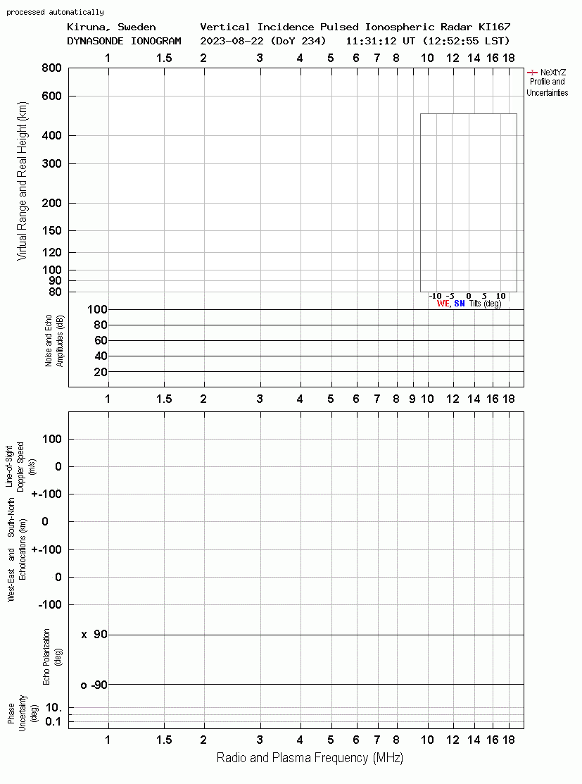
The ionograms appear in two parts (see an example), sharing a common horizontal axis to represent (log) radio and plasma frequencies, f (MHz), and fp (MHz).
Dynasonde R′(f) ionograms are presented in a log-log coordinate system; this provides a constant-percentage display accuracy in both coordinates, and it assists to convey useful detail in the E-region at small ranges and frequency values. It also mitigates the range distortion of «virtual height» in the vicinity of layer penetrations.
The original plots use the full (single-precision) floating-point accuracy of the data processing PC; the graphics system that was used originally («EasyPlot») permits unlimited zooming in these plots, and it is often quite remarkable to witness the smoothness and resolution achieved in (for example) Stationary-Phase Group Range vs radio frequency (where the ultimate resolution is 100 Hz). Of course, zooming accomplishes very little in the GIF images used for Web presentation. But this option is accessible in Java versions of the ionograms, also present on the Web.
In the Dynasonde Ionogram Web Presentation, echo traces (see above) are distinguished by colors (20 are used). Colors are re-cycled in case of necessity by the plotting program, and have no further significance. The same color coding of traces occurs in both parts of one display (and is preserved for all other displays of the same ionogram), but no essential relationship of color exists from one ionogram to another. The traces are also enumerated (1:Jmax) for comparison with the figure legend (and with certain data files), but the enumeration has no significance from one ionogram to another. Trace numerals may be prefixed in several ways: «*» signifies that the trace was selected for the inversion procedure (see below); «<» signifies that the trace was denigrated for the inversion procedure (e.g., Z-traces) or for most other purposes (e.g., «multiple echo» traces). The trace numerals are located at the arithmetic mean frequency and at 90% of the arithmetic mean group height of each trace.
On a secondary Y-axis the «Top 50» calibration curve, the echo decibel amplitude and the pulset mean noise level are plotted versus radio frequency. Decibel amplitudes have no absolute reference: they are simply 10·log(x2 + y2) where x and y are the ADC counts of the receiver quadrature outputs at the echo peak, after compensation for any setting of the receiver»s dynamic step attenuators. The pulset noise level is sampled just before the transmitted pulse; noise values are obtained whether or not echoes are observed, but plotted results occur only for recognized echoes. Method of calculation of the «Top 50» values is explained above. This calculation is done once per day, near 00:00 UT, and is based on the database selection of ionogram echo parameters for preceding 30 days. The «Top 50» calibration curve is the only kind of information shown on an ionogram that represents a result of averaging over long period of time.
As mentioned above, echo classification ultimately depends on a set of attribute-comparison tolerances. Making these tolerances significantly smaller results in more resolution of echolocation, Doppler, etc., and more traces. Significantly larger tolerances reduce the trace count and the resolution of prevailing structure. At present, there is very little dynamic control of these tolerances, but improvements are to be expected with more experience. Some echoes fail to be classified, if (within the tolerances) they are too unlike neighboring echoes; they («UnCl» in the figure legend) are always plotted with small black symbols.
The fp(h) profile is plotted within the ionogram R′(f) log-log coordinates, interpreting the horizontal axis as plasma frequency (see above), and the vertical coordinate as «real» height. The profile inversion procedure assigns model values for two E-F valley parameters (valley width and depth), and permits O and X differential retardations to influence these parameters if they can. Similar control occurs for unobserved nighttime ionization underlying the F-region, using O and X F-region data. As plotted, the F-region profile is extrapolated some distance above the peak, by assuming that near and above the peak it is described by the Chapman law. In the data tables, the sub-peak electron content bTEC is given by integration, and the topside contribution tTEC is estimated from the Chapman layer extrapolation.
The lower part of the ionogram figure contains five phase-dependent echo attributes. For each echo (except recognized «multiple echo» traces and echoes not classified into traces) of the upper part of the figure, there are data points for each attribute in the lower part, and the trace coloring is consistent in the two parts. In descending order, the attributes are:
Echo line-of-sight «Doppler» (or phase-range speed), V* in m/s. This is an average value over the pulset span (.08s for 8-pulsets). Note that expressing «Doppler» in this way removes its dependence on observing frequency or wavelength, so that if a trace represented a frequency-independent «object», V* would appear independent of frequency in these plots. In practice, V* can vary gradually with frequency within traces, and for several possible reasons. Estimation of a trace «Vector Velocity» (Wright and Pitteway, 1994; item 11 of the list above) attempts to combine V* with the line-of-sight direction, over all echoes of a trace in a least-squares process, to determine its intrinsic velocity.
Meridional (magnetic) component of echolocation, YL in km from the zenith, positive Northward; and
Zonal (magnetic) component, XL in km from the zenith, positive Eastward.
These components are from the projection of the direction of arrival of the echo to the group range,
R′. Thus, refraction or deviation from linear
propagation is ignored. By a modernized inversion now in development, we
intend to recover some 3-dimensional ionospheric structure from the
frequency dependence of
XL and YL in a manner analogous to inverting «true» from group range.
Echo polarization rotation, or Chirality, PP (right-side
Y-axis). At all but closely equatorial latitudes, total-reflection echoes are nearly circularly polarized.
PP is the instantaneous phase difference
between Northward- and Eastward-pointing antennas in the dynasonde
receiving array, ~ -90° for
Ordinary-mode echoes, and ~ +90° for eXtraordinary-mode echoes.
At present, the Tromsø receiving array is
unfortunately very near a large crossed-dipole array designed for 2.75
MHz mesospheric studies; the dynasonde «West» receiving antenna is
almost beneath one edge of this array. Some distortion error of
PP near 2.75 MHz is often evident.
Echo Phase Error,
EP (°). The 6 phase-difference echo attributes are determined from 16 phase values in a least-squares estimation;
EP is an error estimate which, multiplied by
factors from the (constant) diagonal elements of the solution covariance
matrix, expresses error-bars or confidence limits on each attribute.
The
table shows these «Confidence Limit Factors» for the 8-pulse pulset in standard use at Tromsø. The
table also shows the equivalent physical attribute dependent on each phase attribute, and the resulting error per degree of
EP.
Usually in dynasonde data processing, an upper limit (currently,
Eplim = 16°) is set to exclude unreliable echoes from further attention. The
figure shows the distribution of
EP from one 11-day sequence in June 1996. The distribution (of log(EP)) is approximately Gaussian, centered on
EP = 1.69°.
It is worthwhile to remark that
EP is usually controlled by «ionospheric
roughness», rather than by such extraneous influences as the
Signal/Noise level or complex-amplitude resolution.
Pitteway, M.L.V. and J.W. Wright, Toward an optimum receiving array and pulse-set for the dynasonde, Radio Science.27, 481-490, 1992
Titheridge, J. E., Ionogram analysis with the generalized program POLAN, Report UAG-93, World Data Center A for Solar-Terrestrial Physics, U.S. Dept. of Commerce, Boulder CO, 80301 USA, 1985.
Wright, J.W. and M.L.V. Pitteway, Real-time data acquisition and interpretation capabilities of the Dynasonde. 1. Data acquisition and real-time display, Radio Sci. 14, 815-825, (1979a)
Wright, J.W. and M.L.V. Pitteway, ...-2. Determination of magnetoionic mode and echolocation using a small spaced receiving array, Radio Sci. 14, 827-835, (1979b)
Wright, J.W. and M.L.V. Pitteway, High-resolution vector velocity determinations from the dynasonde. J. Atmos. Terr. Phys. 56, 961 - 977, 1994.
Wright, J. W. and M. L. V. Pitteway, Data acquisition and analysis for research ionosondes. In Computer Aided Processing of Ionograms and Ionosonde Records, Proc. Session G5 at the XXVth General Assembly of URSI, Lille, France, Aug.28 - Sept. 5, 1996. Ed. by Phil Wilkinson. Report UAG 105, NGDC, NOAA, 325 Broadway, Boulder, CO, 80303 USA.
Wright, J. W. and M. L. V. Pitteway, A new data acquisition concept for digital ionosondes: Phase-based echo recognition and real-time parameter estimation. Radio Science 34, 871-882, 1999.
Zabotin, N. A. and J. W. Wright, Ionospheric irregularity diagnostics from the phase structure functions of MF / HF radio echoes. Radio Science 36, 757-771, 2001